Pathfinding algorithms are one of the most important subjects of computer science. They are used in fields such as video games, geography information systems, and networking. They depend on Graph Theory.

Pathfinding algorithms are used for different purposes like finding the shortest route to reduce fuel consumption, calculating the most suitable way for an AI character that belongs to a video game, redirecting network packages to the best way possible, etc.

These algorithms may have so many different variations and they could get so many different parameters according to the circumstances. The shortest way might not be the best way. If a pathfinding algorithm is calculating a path, it should also consider traffic, road work, roads in poor condition, hills, tolls, bridges, etc. Otherwise, it could cause more harm than good. So, finding the best way might be more important than finding the shortest way.

These representations are made with graphs. For example, A, B, C are cities and they are called "nodes". Roads are edges. This graph is an undirected graph. Because the edges are both inbound and outbound. It is also cyclic. Because the graph is closed.



If this graph was an open graph, it could be an acyclic graph.


If there was a one-way trip, it could be a directed graph.


One of the most important sides of the undirected graph is round-trip can be represented with different weights. For example, the altitude of City B might be higher than the altitude of City C, and going from City B to City C could be easier than going from C to B. Because going down is easier. Therefore, if the value given to going City B to City C is 4 units, the value of returning from City C to City B can be expressed as 5 units.


While finding the shortest route is very critical for airline companies because of fuel consumption, this is not so important for video games. Choosing a faster pathfinding algorithm that finds a slightly longer route for a video game character may also look more natural. In real life, people and animals tend to choose the shortest path but they cannot measure the road precisely and they cannot know every detail, obstacle, etc. So, they cannot compute the shortest path like a computer. Their chosen path is intuitive.

Finding the shortest path might take so much time, depending on the vertex and edge count. The algorithm complexity might also increase that time, dramatically. So, video games use intuitive pathfinding algorithms more than the algorithms that find the exact shortest path. Maybe the game character may choose a longer path. But the game performance will be better.

At this point, A* algorithm is very useful. The algorithm can successfully calculate a short path, depending on the quality of the heuristic function. But I would like to talk about Dijkstra's Algorithm before A* Algorithm.  Because they are so similar but Dijkstra's Algorithm has no heuristics.

Let,

A*;
f(x) = g(x) + h(x)

Dijkstra;
f(x) = g(x)

g: Real distance
h: Intuitive distance

In short, Dijkstra calculates the precise route, A* calculates the approximation.

Now, I will explain it with some C++ code after talking about defining graphs in memory.

First of all, I will talk about the ways to store edges (interconnection of vertices) in memory. The first one is "Adjacency List", and the second one is "Adjacency Matrix".

Graph



Adjacency List
Adjacency Matrix


Both of them have some advantages and disadvantages over each other. If the graph is represented by an adjacency matrix, writing code and accessing the values are easier. But the matrix also keeps some unrelated vertex connection info and this takes some memory.

If the graph is represented by an adjacency list, it takes more time to develop but only necessary memory will be used. If you have a huge graph, this is a crucial fact that cannot be ignored.

I will use Adjacency List in my article. Because, in some cases, memory consumption may be very important.

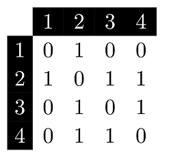
Adjacency List: Every vertex has a linked list and if there is a connection, we add the neighbour vertex to that list. For example, if we look at the 2's linked list, we see 1, 3, 4 as its neighbours.

Adjacency Matrix: As it seems, in the Adjacency Matrix, vertices are represented by rows and columns. This graph is not a weighted graph. So, all values are 0 (Not connected) or 1 (Connected). For example, we go to row 1 and look at column 2 to see if there is a link from 1 to 2. Since there is 1, this means there is a connection.


Now, I start with the definition of a vertex in C++.
1
struct Vertex {
2
  int weight;
3
  int dest;
4
};

As it seems, Vertex is a structure that keeps weight and destination. Weight keeps the distance and Destination keeps the number of the neighbour vertex. If you look at the graph that is below, you will see that dest is 2, weight is 4.



And, we are beginning to define the Graph class.
1
class Graph {
2
 private:
3
  list<Vertex*> *adjList;
4
  int vCount;
5
 public:
6
  ...

We keep Adjacency List ("adjList") as a Vertex pointer list. The "list" data structure belongs to STL. vCount keeps the number of vertices.


We define the constructor part,
1
explicit Graph(int vCount) {
2
  adjList = new list<Vertex*>[vCount];
3
  this->vCount = vCount;
4
}
In this constructor, we create lists according to vCount (Vertex Count) and store the vCount's value.

Note: We store the vertex pointers in the lists, do not forget to deallocate them in the destructor function.


Now, we are adding vertices and edges,
1
Vertex* createVertex(int dest, int weight) {
2
  Vertex* newVertex = new Vertex;
3
  newVertex->dest = dest;
4
  newVertex->weight = weight;
5
  return newVertex;
6
}
7
 
8
void addEdge(int src, int dest, int weight) {
9
  Vertex* newVertex = createVertex(dest, weight);
10
  adjList[src].push_back(newVertex);
11
 
12
  /*newVertex = createVertex(src, weight);
13
  adjList[dest].push_back(newVertex);*/
14
}
In the createVertex function, we created a new vertex, we assigned dest and weight info and returned the pointer.

In the addEdge function, we use the createVertex function to create the neighbour vertex first, we get the source vertex's list and add the newly created neighbour vertex's pointer to the list. This creates a directed graph. If you want to create an undirected graph, comment out the commented lines.


This is an example to use the graph class,
1
Graph g(4);
2
g.addEdge(0, 1, 3); // 0->1 (3)
3
g.addEdge(0, 2, 2); // 0->2 (2)
4
g.addEdge(1, 2, 3); // 1->2 (3)
5
g.addEdge(2, 3, 5); // 2->3 (5)
6
g.addEdge(3, 0, 2); // 3->0 (2)

It is time to talk about traversing on a graph. Before this, we could look at the binary tree traversing methods. DFS (Depth-first search) and BFS (Breadth-first search). DFS is a top-down recursive approach. BFS is visiting all neighbours of a vertex first. So, BFS is useful for our task.

Depth-first Search


Breadth-first Search


This is our BFS function to traverse the graph,
1
void bfs(int index) {
2
  bool* visited = new bool[vCount];
3
 
4
  for (int i = 0; i < vCount; i++) {
5
    visited[i] = false;
6
  }
7
 
8
  // Add the first vertex to the queue
9
  queue<int> q;
10
  q.push(index);
11
  visited[index] = true;
12
 
13
  // While the queue is not empty, continue
14
  while (!q.empty()) {
15
    int current = q.front();
16
    q.pop();
17
 
18
    cout << current << endl;
19
 
20
    // Get the neighbours
21
    list<Vertex*> neighbours = adjList[current];
22
   
23
    list<Vertex*>::iterator itr;
24
    for (itr = neighbours.begin(); itr != neighbours.end(); itr++) {
25
      int destIndex = (*itr)->dest;
26
    
27
      // If the neighbour is not visited, add it to the list  
28
      if (!visited[destIndex]) {
29
        q.push(destIndex);
30
        visited[destIndex] = true;
31
      }
32
    }
33
  }
34
 
35
  delete[] visited;
36
}
In our BFS algorithm, we visit the neighbours of the vertex and use a STL queue to keep vertices.

We keep the visit info in the "visited" array not to cause a forever loop if there is a cyclic graph.

At first, we push the index of the first vertex in the queue for initialization, later we pop it from the queue. we access the neighbours of the vertex and we push the neighbour's index if it is not visited. If it is not visited, we mark it as visited. If the queue is empty, it is done. This is the summary.


Now, we can talk about Dijkstra's Algorithm. As I said, this algorithm gives the precise answer. It is not heuristic. So, it takes more time. If we develop a game, we don't need the exact solution. We need an approximation. But I will also mention Dijkstra's Algorithm. A* Algorithm is similar to Dijkstra's Algorithm.

1
void dijkstra(int index) {
2
  unsigned int* distance = new unsigned int[vCount];
3
  bool* visited = new bool[vCount];
4
 
5
  for (int i = 0; i < vCount; i++) {
6
    distance[i] = -1;
7
    visited[i] = false;
8
  }
9
 
10
  // Defined priority queue for optimization
11
  priority_queue<iPair, std::vector<iPair>, CompareVertexDistances> pq;
12
  
13
  // Add the first vertex to the queue
14
  pq.push(pair<int, int>(index, 0));
15
  distance[index] = 0;
16
  visited[index] = true;
17
 
18
  // While the queue is not empty, continue
19
  while (!pq.empty()) {
20
    cout << pq.top().second << endl;
21
    int currentIndex = pq.top().first;
22
    list<Vertex*> neighbours = adjList[currentIndex];
23
    pq.pop();
24
 
25
    list<Vertex*>::iterator itr;
26
    for (itr = neighbours.begin(); itr != neighbours.end(); itr++) {
27
      int destIndex = (*itr)->dest;
28
      if (!visited[destIndex]) {
29
        unsigned int temp = distance[currentIndex] + (*itr)->weight;
30
 
31
        if (distance[destIndex] > temp) {
32
          distance[destIndex] = temp;
33
        }
34
 
35
        pq.push(iPair(destIndex, distance[destIndex]));
36
        visited[destIndex] = true;
37
      }
38
    }
39
  }
40
 
41
  // List the distances
42
  for (int i = 0; i < vCount; i++) {
43
    cout << distance[i] << endl;
44
  }
45
 
46
  delete[] visited;
47
  delete[] distance;
48
}
We used BFS here again.

In Dijkstra's algorithm, we also used a distance array besides the visited array. For the first vertex, the distance is zero. This represents the distance to itself. We set the others -1. In Dijkstra Algorithm, this -1 actually represents infinite. But we cannot define infinite on a computer. So, we use the highest possible unsigned value. If we assign -1 to an unsigned 32 bit variable, it will be 0xFFFFFFFF. If we assign -1 to an unsigned 64 bit variable, it will be 0xFFFFFFFFFFFFFFFF. You could also use "climits" to define the maximum value, alternatively.

These distance values will be updated while we are traversing. Small values will overwrite large values and we will find the shortest route.

The standard Dijkstra Algorithm's complexity is . The optimized Dijkstra Algorithm's complexity is . To achieve optimization, we use priority_queue instead of queue. C++ STL also includes a priority queue. If there wasn't a priority queue in C++ Standard Template Library (STL), we could design a min-heap data structure. In min-heap, a parent node keeps a lower number than its children. In max-heap, it is the opposite.

Min-Heap


Max-Heap


Priority Queue put the elements in order from biggest to smallest in default. We need its opposite. So, we will add a custom comparison function for Priority Queue. It will put the elements in order from smallest to biggest now. We will use vertex index, distance pair as a parameter. We need this info for comparison and we will define iPair for writing shorter code later. 

1
typedef pair<int, int> iPair;
This is our comparison class.

1
class CompareVertexDistances {
2
 public:
3
  bool operator()(const pair<int, int>& v1, const pair<int, int>& v2) {
4
    if (v1.second > v2.second)
5
      return true;
6
    else
7
      return false;
8
  }
9
};

Finally, it is time to talk about A* Algorithm. We mentioned everything needed. This algorithm's difference is it is intuitive.

In A* Algorithm, we will use a grid view and we won't only consider roads. We will mark the obstacle locations as not usable.

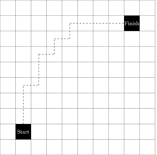Every vertex has x, y coordinates on this grid. We will measure the distance by using these.

There are two different heuristic approaches that we could use here. Manhattan Distance and Euclidean Distance.

Manhattan Distance
1
int getManhattanDistance(const Vertex& start, const Vertex& end) {
2
  int distX = abs(start.x – end.x); // X difference
3
  int distY = abs(start.y – end.y); // Y difference
4
  
5
  return D * (distX + distY); // D is the step value. Moving to neighbour requires 1 step.
6
}
It is quite useful if you are working on a grid.

The other one is Euclidian Distance (). The game character uses every direction not just the perpendicular directions.

Euclidian Distance
1
int getEuclideanDistance(const Vertex& start, const Vertex& end) {
2
  int distX = abs(start.x – end.x);
3
  int distY = abs(start.y – end.y);
4
  
5
  return D * sqrt(dx*dx + dy*dy); // D is the step value. Moving to neighbour requires 1 step.
6
}

These were our A* Algorithm heuristic functions.

At this point, we can modify our code and also add finishIndex. We don't need to deal with every vertex to get a good result. If we reach finishIndex, we end the operation.

1
void aStar(int startIndex, int finishIndex) {
2
...
If currentIndex equals to finishIndex, we end the operation.

1
...
2
 
3
while (!pq.empty()) {
4
  cout << pq.top().second << endl;
5
  int currentIndex = pq.top().first;
6
 
7
  if(currentIndex == finishIndex)
8
    break;
9
 
10
  list<Vertex*> neighbours = adjList[currentIndex];
11
  pq.pop();
12
 
13
...
We modify our Priority Queue to add Manhattan Distance Heuristic function.

1
...
2
pq.push(iPair(destIndex, distance[destIndex] + getManhattanDistance(currentVertex, finishVertex)));
3
...

And it is done. We have an A* algorithm. It is a quite effective algorithm for video games. We might use the other variations of it as well. This is the standard implementation.